OVERVIEW: The premise is that changes in the value of a main variable (for example, the sales of Product A) are closely associated with changes in some other variable(s) (for example, the cost of Product B). So, if future values of these other variables (cost of Product B) can be estimated, it can be used to forecast the main variable (sales of Product A).
BASIC IDEA: Regression analysis is a statistical technique for quantifying the relationship between variables. In simple regression analysis, there is one dependent variable (e.g. sales) to be forecast and one independent variable. The values of the independent variable are typically those assumed to "cause" or determine the values of the dependent variable. Thus, if we assume that the amount of advertising dollars spent on a product determines the amount of its sales, we could use regression analysis to quantify the precise nature of the relationship between advertising and sales. For forecasting purposes, knowing the quantified relationship between the variables allows us to provide forecasting estimates.
PROCEDURE: The simplest regression analysis models the relationship between two variables uisng the following equation: Y = a + bX, where Y is the dependent variable and X is the independent variable. Notice that this simple equation denotes a "linear" relationship between X and Y. So this form would be appropriate if, when you plotted a graph of Y and X, you tended to see the points roughly form along a straight line (as compared to having a curvilinear relationship).
When you have several past concurrent observations of Y and X, regression analysis provides a means to calculate the values of a and b, which are assumed to be constant. Since you will then know a and b, if you can provide an estimate of X in some future period, you can calculate a future value of Y from the above equation.
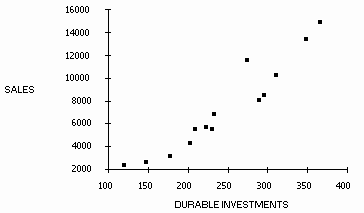
EXAMPLE: We can illustrate regression analysis using data from 1976-1989 for both the annual value of sales of semiconductors (in $M) and a likely leading indicator of these sales, namely Producers' durable equipment investment (in $B). First, a graph of the relationship between these two variables suggests that they might be related in a linear fashion:

We can run a regression of sales on durable equipment investment, which has an equation that looks like this:
Sales = a + b (Investment)
Using this data, we get the following results:
Sales = -5513.7 + 52.3 (Investment)
t=4.4 t=10.7
The last line are the "t-statistics" for the estimate of a (which is -5513.7) and b (which is 52.3). These t-statistics allow you to test whether the estimates are significantly different from 0. If the estimate is not different from 0, then it should be considered 0 when using the regression equation for a forecast (see below). This is a distinct advantage of regression analysis because it allows you to assess whether the linear relationship might have occurred by chance (most of the other techniques don't do this!).
As a quick rule of thumb, if the number of observations is between 5 and 20, a t greater than 3 assures that your estimate is significantly greater than 0 with a confidence of 95%. If the number of observations is greater than 20, a t greater than 2 is good enough. In the above example, our estimates of a and b are both significantly greater than 0.
To make a forecast, lets assume we that the leading indicator estimate for Producers' durable equipment investment for next year is 370. Plugging this into the above equation, our forecast would be:
Sales = -5513.7 + 52.3 (370) = 13,837
Note that if our estimate of "a" was not statistically significant (i.e. t<3), then we would calculate next period's forecast of Sales as:
Sales = 0 + 52.3 (370) = 19,351
COMMENTS:
• More complicated relationships between variables can be readily modeled. For example, several independent variables can be incorporated into the analysis or curvilinear relationships can be handled.
• When the independent variable is "time", you get an estimate of the trend line for a time series. The resulting equation is: Sales = -66841.3 + 898.8 (time). This suggests that the underlying "trend" of this data is approximately 898.8$B per year.
• Many analysts plot data using the logarithm of the dependent variable - for example, using the log (sales) versus time. If this approach results in a graph with points that roughly form along a straight line, a reasonable model for approximating the data is: log(sales) = a + b(time). This presents no problem since you then run a regression of log (sales) on time and interpret the estimate for b as the trend grwoth rate associated with the logarithm of sales.
• Forecasting accuracy heavily depends on the accuracy of the estimates for the independent variable.
• A consistent relationship between the variables is assumed when making forecasts. This, of course, may not be the case in many situations.
• Provides statistical tests and confidence intervals for the actual forecasts which most quantitative techniques lack.
